Als erfahrener Google-Sheets-Experte mit Jahren der Praxis in der Tabellenoptimierung weiß ich: Die Anzeige der aktuellen Uhrzeit ist eine der nützlichsten Funktionen. Für Einsteiger mag die Syntax zunächst verwirrend wirken, doch es ist kinderleicht.

In diesem praxisnahen Guide zeige ich Ihnen Schritt für Schritt, wie Sie mit den bewährten Funktionen JETZT() und HEUTE() die aktuelle Zeit, Uhrzeit oder beides einbinden. Passen Sie das Ergebnis flexibel an – ideal für Buchhaltung, Projektmanagement oder tägliche Reports. Vertrauen Sie auf meine bewährten Methoden, die ich in Dutzenden Projekten erfolgreich eingesetzt habe.
Hier die detaillierten Anweisungen für die gängigsten Ansätze.
Aktuelle Uhrzeit und Datum mit JETZT() einfügen
Die Funktion JETZT() ist mein Go-to-Tool für präzise Zeitstempel. Sie liefert Datum und Uhrzeit in Echtzeit und lässt sich nahtlos in Formeln integrieren.
Syntax: =JETZT()
Keine Argumente nötig – einfach und effizient. Perfekt für genaue Logs in Finanz- oder Arbeitszeit-Tabellen.
- Öffnen Sie eine Google-Tabelle oder erstellen Sie eine neue.
- Klicken Sie auf die gewünschte Zelle, um sie zu aktivieren.
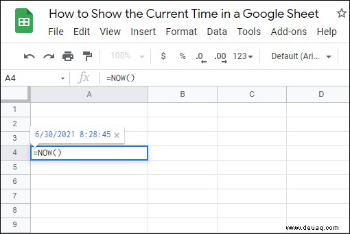
- Geben Sie
=JETZT()ein und drücken Sie Enter. Das aktuelle Datum und die Uhrzeit erscheinen sofort. Die Formel sehen Sie in der Bearbeitungsleiste.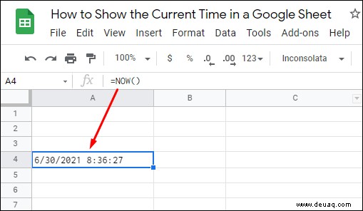
Wichtige Fakten zur JETZT()-Funktion:
- Sie ist flüchtig: Aktualisiert sich bei jeder Neuberechnung (z. B. jede Minute oder Stunde, einstellbar in den Tabellenoptionen).
- Zeigt immer die aktuelle Zeit nach Neuberechnung, nicht den Einstiegszeitpunkt.
- Formatieren Sie die Zelle, um nur Datum oder Uhrzeit zu zeigen.
Nur das aktuelle Datum mit HEUTE() anzeigen
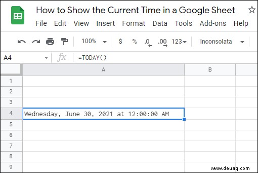
Für reines Datum ohne Uhrzeit: Nutzen Sie HEUTE(). Das Format passt sich Ihren lokalen Einstellungen an (z. B. TT.MM.JJJJ).
Syntax: =HEUTE() – ebenfalls ohne Argumente.
- Wählen Sie eine leere Zelle aus.
- Geben Sie
=HEUTE()ein und drücken Sie Enter.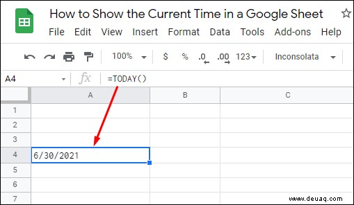
Die Zelle aktualisiert sich täglich. Passen Sie das Format nach Bedarf an.
Formatierung von Datum- und Uhrzeitformeln optimieren
Standardmäßig zeigt JETZT() beides an. Ändern Sie das mühelos über die Formatierung – gilt auch für HEUTE().
- Markieren Sie die Zelle mit der Formel.
- Klicken Sie auf Format in der Menüleiste.
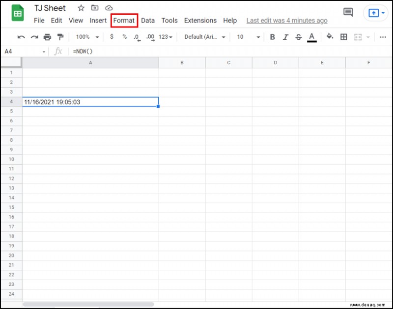
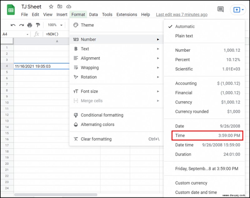
- Wählen Sie Zahl aus dem Dropdown.
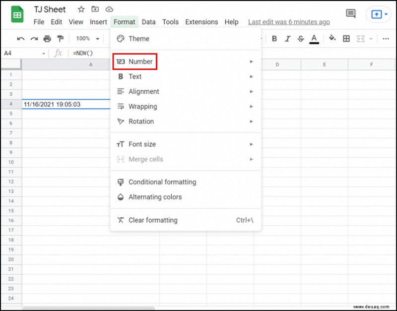
- Für reine Uhrzeit: Uhrzeit; für Datum: Datum.
Für erweiterte Optionen:
- Markieren Sie Zelle(n).
- Format > Zahl > Weitere Formate > Weitere Datums- und Uhrzeitformate.
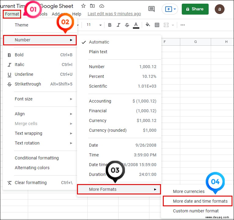
- Wählen Sie aus Dutzenden Vorlagen (z. B. mit Text, Schrägstrich) und klicken Sie Anwenden.
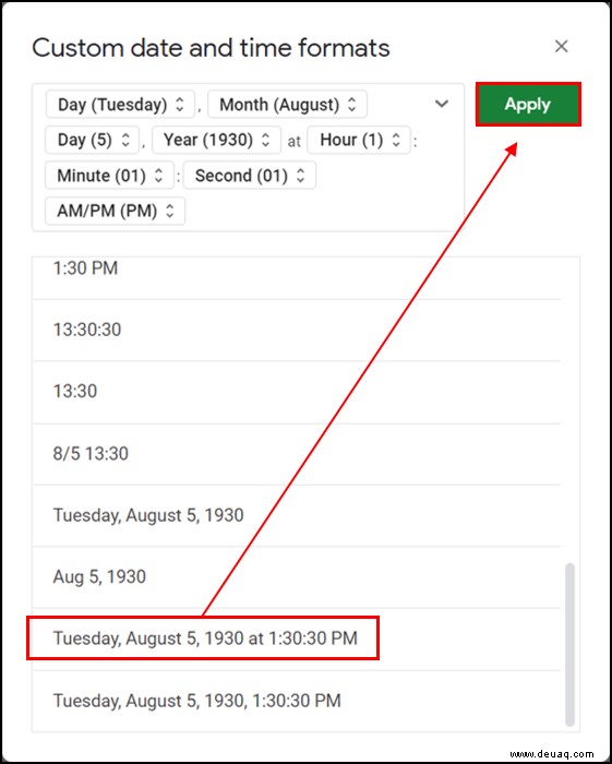
- Überprüfen Sie das Ergebnis.
Verschiedene Formate pro Zelle? Kein Problem!
Zusätzliche FAQs
Statische Datum/Uhrzeit einfügen?
Für feste Werte (nicht flüchtig):
- Windows: Strg + ; (Datum), Strg + Umschalt + : (Uhrzeit + Datum)
- Mac: Cmd + ; (Datum)
JETZT() und HEUTE() können keine statischen Werte erzeugen.
GoogleClock noch nutzbar?
Nein, veraltet. Verwenden Sie stattdessen JETZT() oder HEUTE() – zuverlässiger für alle Sheets.
Uhrzeit in Dezimalzahlen umwandeln?
Ja, z. B. für Arbeitszeiten. Nutzen Sie STUNDE(), MINUTE(), SEKUNDE() oder ZEITWERT().
STUNDE(zeit): Extrahiert Stunden, z. B. aus "05:14:40" → 5.=STUNDE(B3)
MINUTE(zeit): Minuten, z. B. → 14.=MINUTE(B3)
SEKUNDE(zeit): Sekunden, z. B. → 40.=SEKUNDE(B3)
In Stunden dezimal: =STUNDE(B3)+MINUTE(B3)/60+SEKUNDE(B3)/3600
In Minuten: =STUNDE(B3)*60+MINUTE(B3)+SEKUNDE(B3)/60
In Sekunden: =STUNDE(B3)*3600+MINUTE(B3)*60+SEKUNDE(B3)
Zeit ist Geld – nutzen Sie sie weise
Mit diesem Guide beherrschen Sie Zeitstempel in Google Sheets. Ob Analyst oder Alltagsnutzer: JETZT() und HEUTE() sparen Stunden.
Wie setzen Sie die Funktionen ein? Teilen Sie Erfahrungen in den Kommentaren!